Fundamentals of SQL Window function
Window functions provide the ability to perform calculations across a set of rows that are related to the current row. Window functions can help solve various querying tasks by helping you express set calculations more quickly, intuitively, and efficiently. They are mainly used for analytical purposes because they allow you to perform many computations.
In this first article of this series, I will go through the concept of the window function. I will be using PostgreSQL for the entire series, but the concept should apply to other RDMS. The dataset I use is the Chinook database.
Introduction
A window function call always has an OVER clause directly after the window function's name and arguments, which distinguishes it from a regular aggregate function. Below is the structure of a typical window function query.
SELECT <colum 1>, <column 2>, ...
       <window function>() OVER (
           PARTITION BY <...>
           ORDER BY <...>
           <window frame>
       );
PARTITION BY, ORDER BY, and window frame definition are all optional.
The following example shows the rank of total sales grouped by customers using the DENSE_RANK window function.
SELECT invoice.customer_id,
       customer.first_name,
       customer.last_name,
       SUM(total),
       DENSE_RANK() OVER (ORDER BY SUM(total) DESC)
FROM invoice
INNER JOIN customer ON invoice.customer_id = customer.customer_id
GROUP BY invoice.customer_id, customer.first_name, customer.last_name;
 customer_id | first_name | last_name  |  sum  | dense_rank
-------------+------------+------------+-------+------------
           6 | Helena     | Holý       | 49.62 |          1
          26 | Richard    | Cunningham | 47.62 |          2
          57 | Luis       | Rojas      | 46.62 |          3
          45 | Ladislav   | Kovács     | 45.62 |          4
          46 | Hugh       | O'Reilly   | 45.62 |          4
          28 | Julia      | Barnett    | 43.62 |          5
          37 | Fynn       | Zimmermann | 43.62 |          5
         <------------------ TRUNCATED -------------------->
We can also use the named window shown below.
SELECT <colum 1>, <column 2>
       <window function>() OVER <window_name>
FROM <table_name>
WHERE <...>
GROUP BY <...>
HAVING <...>
WINDOW <window_name> AS (
   PARTITION BY <...>
   ORDER BY <...>
   <window frame>)
ORDER BY <...>;
We can modify our earlier query to using the named window shown below.
SELECT invoice.customer_id,
       customer.first_name,
       customer.last_name,
       SUM(total),
       DENSE_RANK() OVER dense_rank_window
FROM invoice
INNER JOIN customer ON invoice.customer_id = customer.customer_id
GROUP BY invoice.customer_id, customer.first_name, customer.last_name
WINDOW dense_rank_window as (
   ORDER BY SUM(total) DESC
);
The result is identical to the unnamed window definition example.
Window function vs. normal aggregate function
A Window function looks similar to aggregation. However, unlike aggregate functions, window functions do not collapse rows and instead, the rows retain their identities.
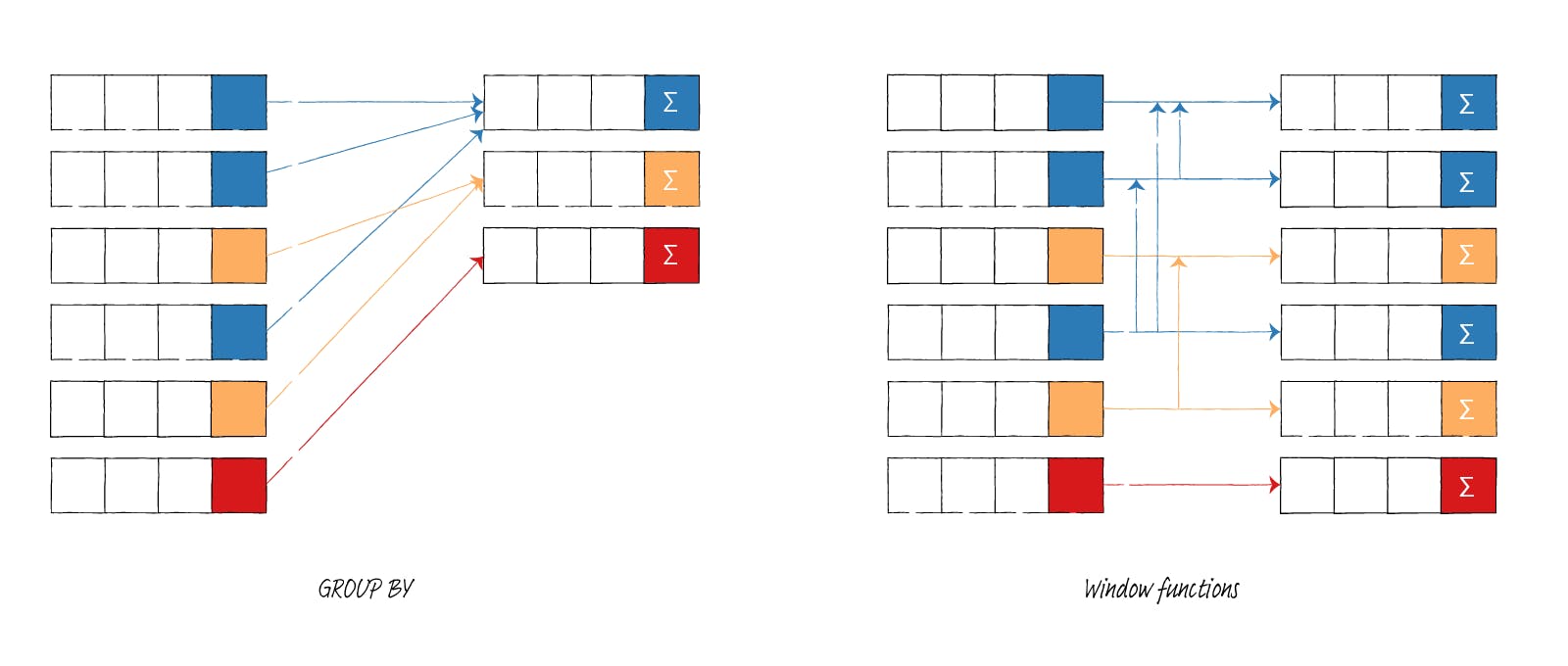
Because window functions do not collapse rows, window functions are great alternatives for aggregations, regular aggregations give you insight, but you also lose some detail.
When to use window functions
You should use windows functions to compute values for each result set row that depends on other rows within the same result set. Some typical use cases for using window functions are
- Fetching preceding or following rows
- Assigning ordinal rank to rows
- Calculate running total
- Calculate moving average
A classic example is a sales analysis of weekly results where you need to output both each day's gross sales and the variation with the same day compared to the previous week.
Logical order for window functions
To understand window functions better, we should learn about the order of operation in SQL. Below is the logical order of operations in SQL.
- FROM, JOIN
- WHERE
- GROUP BY
- Aggregate functions
- HAVING
- Window functions
- SELECT
- DISTINCT
- UNION/INTERSECT/EXCEPT
- ORDER BY
- OFFSET
- LIMIT/FETCH/TOP
You can use window functions on SELECT and ORDER BY statements. But you can't put window functions anywhere in the FROM, WHERE, GROUP BY, or HAVING clauses.
The critical consequence of this logical order is that rows considered by a window function are those of the "virtual table" or result from sets filtered by its WHERE, GROUP BY, and HAVING clauses if any. If a WHERE condition removes a row, the window function will not see it.
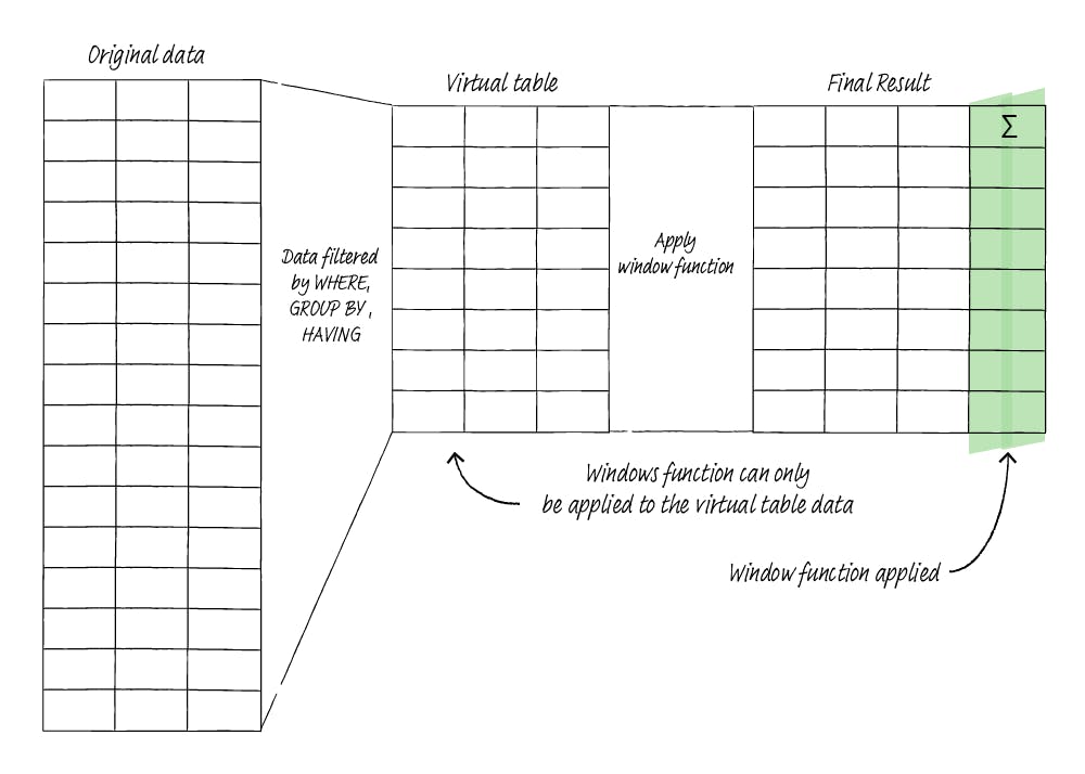
How window function operates
Window functions operate on three things: partition, order, and frame.
Partition
You use partition to divide rows into multiple groups. Once you group rows into sections, you can then apply window functions.

The PARTITION BY clause inside OVER divides the rows into sections that share the same values as the PARTITION BY expressions. The window function is calculated across the rows inside the same partition as the current row.
The following query will partition customers by billing _city and generate the total sum for that city.
SELECT customer_id,
       billing_city,
       total,
       SUM(total) OVER(PARTITION BY billing_city)
FROM invoice;
customer_id | billing_city | total |  sum
-------------+--------------+-------+-------
          48 | Amsterdam    |  1.98 | 40.62
          48 | Amsterdam    | 13.86 | 40.62
          < ..........TRUNCATED.......... >
          59 | Bangalore    |  1.99 | 36.64
          59 | Bangalore    |  8.91 | 36.64
          < ..........TRUNCATED.......... >
          38 | Berlin       |  1.98 | 75.24
          38 | Berlin       | 13.86 | 75.24
          < ..........TRUNCATED.......... >
If you do not specify any PARTITION BY clause, the entire result set is the partition.
Order
We can order the rows in each partition using ORDER BY before applying a window function.
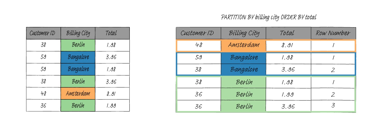
When we do not specify ORDER BY, the order of rows within each partition is arbitrary.
The following query partitioned the data by billing city and added a number for each row within the partition.
SELECT customer_id,
       billing_city,
       total,
       ROW_NUMBER() OVER(PARTITION BY billing_city ORDER BY total)
FROM invoice;
customer_id |    billing_city     | total | row_number
-------------+---------------------+-------+------------
          48 | Amsterdam           |  0.99 |          1
          48 | Amsterdam           |  1.98 |          2
         < ..................TRUNCATED................. >
          59 | Bangalore           |  1.98 |          1
          59 | Bangalore           |  1.99 |          2
         < ..................TRUNCATED................. >
          38 | Berlin              |  0.99 |          1
          36 | Berlin              |  0.99 |          2
          36 | Berlin              |  1.98 |          3
         < ..................TRUNCATED................. >
Frame
A window frame specifies the set of rows to be included in our computation. The window frame is examined separately within each partition, giving us a subset of each partition.
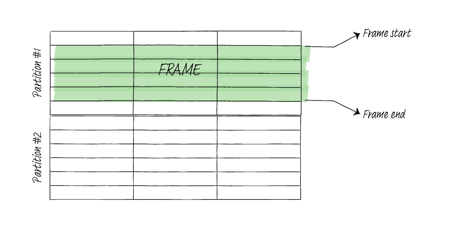
Frames are defined using bounds, and it runs from the frame start to the frame end. If you don't specify frame end, the end defaults to CURRENT ROW. The frame start must be before the frame end.
The bounds are:
- UNBOUNDED PRECEDING
- n PRECEDING
- CURRENT ROW
- n FOLLOWING
- UNBOUNDED FOLLOWING
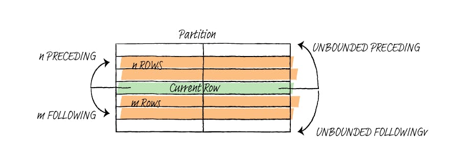
You can specify the bounds in RANGE, ROWS, or GROUPS mode. To better illustrate the difference between them, let's run the following query:
SELECT customer_id as cid,
       billing_city as city,
       total,
       SUM(total) OVER(PARTITION BY billing_city
                       ORDER BY total) AS DEFAULT,
       SUM(total) OVER(PARTITION BY billing_city
                       ORDER BY total
                       ROWS BETWEEN 1 PRECEDING AND 1 FOLLOWING) AS rows,
       SUM(total) OVER(PARTITION BY billing_city
                       ORDER BY total
                       RANGE BETWEEN 1 PRECEDING AND 1 FOLLOWING) AS range,
       SUM(total) OVER(PARTITION BY billing_city
                       ORDER BY total GROUPS
                       BETWEEN 1 PRECEDING AND 1 FOLLOWING) AS groups
FROM invoice;
 cid |  city  | total | default | rows  | range | groups
-----+--------+-------+---------+-------+-------+--------
 <----------------------- TRUNCATED --------------------->
  36 | Berlin |  0.99 |    1.98 |  1.98 |  9.90 |   9.90
  38 | Berlin |  0.99 |    1.98 |  3.96 |  9.90 |   9.90
  36 | Berlin |  1.98 |    9.90 |  4.95 |  9.90 |  17.82
  36 | Berlin |  1.98 |    9.90 |  5.94 |  9.90 |  17.82
  38 | Berlin |  1.98 |    9.90 |  5.94 |  9.90 |  17.82
  38 | Berlin |  1.98 |    9.90 |  7.92 |  9.90 |  17.82
  36 | Berlin |  3.96 |   17.82 |  9.90 |  7.92 |  27.72
  38 | Berlin |  3.96 |   17.82 | 13.86 |  7.92 |  27.72
  36 | Berlin |  5.94 |   29.70 | 15.84 | 11.88 |  37.62
  38 | Berlin |  5.94 |   29.70 | 20.79 | 11.88 |  37.62
  36 | Berlin |  8.91 |   47.52 | 23.76 | 17.82 |  57.42
  38 | Berlin |  8.91 |   47.52 | 31.68 | 17.82 |  57.42
  38 | Berlin | 13.86 |   75.24 | 36.63 | 27.72 |  45.54
  36 | Berlin | 13.86 |   75.24 | 27.72 | 27.72 |  45.54
 <----------------------- TRUNCATED --------------------->
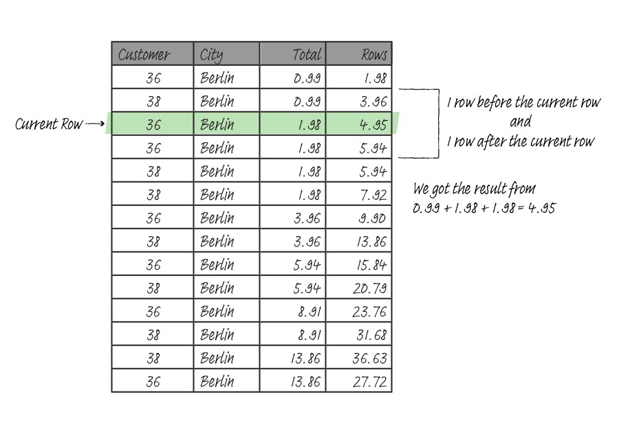
ROWS
The ROWS mode treats every row as a distinct row, even when the value is duplicated. If you need to define an arbitrary size for a window frame, you must use ROWS, which enables you to input how many rows (preceding or following) are to be included in the window frame.
RANGE
The RANGE mode requires an ORDER BY clause that specifies precisely a single column. The actual rows included in the frame depend on the maximum difference between the column's value in the current row with preceding or following offset. Offset is just a fancy name for the n in the n PRECEDING or n FOLLOWING statement.
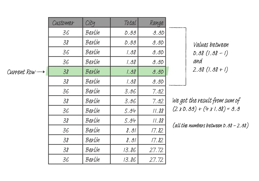
In RANGE mode, the offset depends on the data type of the ordering column. Suppose you use numeric columns as the ordering column, then your offset will be the same type as the ordering column. For example, if your ordering column is type numeric, you would write RANGE BETWEEN 1 PRECEDING AND 1 FOLLOWING. But if your ordering column data type is date or timestamp, you would need to use an interval. Something like, RANGE BETWEEN '2 days' PRECEDING AND '2 days' FOLLOWING.
GROUPS
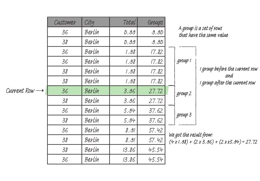
In GROUPS mode, the frame start is specified by the number of a peer group before the current's row peer group and ends with the following peer group. A peer group contains rows that have the same value as an ORDER BY ordering. Like in RANGE mode, you must have an ORDER BY clause to use GROUPS mode.
Default window frame
If you do not explicitly specify the frame, the default window frame must follow the following rules:
- If an ORDER BY is specified, then the frame is RANGE BETWEEN UNBOUNDED PRECEDING AND CURRENT ROW
- If an ORDER BY is NOT specified, then the frame uses the whole set of rows. In other words, it is bound between UNBOUNDED PRECEDING and UNBOUNDED FOLLOWING.
Wrap up
In this article, I have laid down the fundamental concept of window functions. In the following article, I will explain all of the available window functions with some examples.
